biasutti2019riu

Module that implements the model from RIU-Net: Embarrassingly simple semantic segmentation of 3D LiDAR point cloud.

Summarizing quotes from the paper:

1. Introduction

• “we propose RIU-Net (for Range-Image U-Net), the adaptation of U-Net […] to the semantic segmentation of 3D LiDAR point clouds.” ### 2. Related works
• “Recently, Wu et al. proposed SqueezeSeg, a novel approach for the semantic segmentation of a LiDAR point cloud represented as a spherical range-image.” ### 3. Methodology
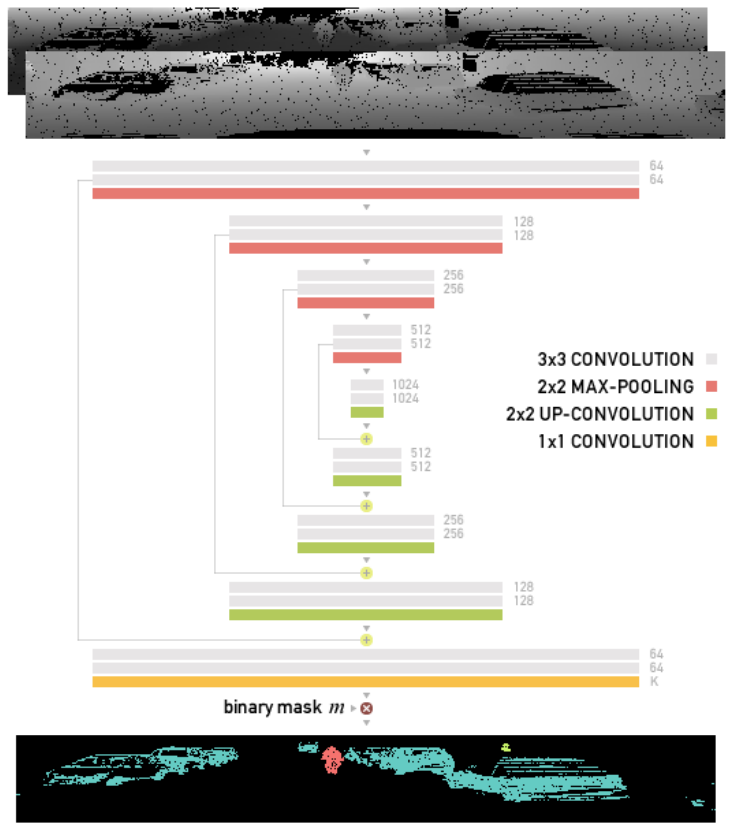
• “The method consists in feeding the U-Net architectures with 2-channels [range-images] encoding range and elevation.” #### 3.A Input of the Network
• “we use a range-image named u of 512 × 64px with two channels: the depth towards the sensor and the elevation.”
• “We propose to identify [empty pixels (pixels that are considered invalid by the LIDAR sensor)] using a binary mask m equal to 0 for empty pixels and to 1 otherwise.” #### 3.B Architecture
• “the encoder consists in the repeated application of two 3×3 convolutions followed by a rectified linear unit (ReLU) and a 2×2 max-pooling layer that downsamples the input by a factor 2. Each time a downsampling is done, the number of features is doubled.”
• “The decoder consists in upsampling blocks where the input is upsampled using 2 × 2 up-convolutions. Then, concatenation is done between the upsampled feature map and the corresponding feature map of the encoder. After that, two 3 × 3 convolutions are applied followed by a ReLU. This block is repeated until the output of the network matches the dimension of the input.”
• “the last layer consists in a 1x1 convolution that outputs as many features as the wanted number of possible labels K 1-hot encoded.” #### 3.C Loss function
• “is defined as the cross-entropy of the softmax of the output of the network.”

\[ E = -\sum_{x \in \Omega}{ \mathbf{1}_{\{m(x)>0\}}w(x)\log(p_{l(x)}(x))} \]

• “[in the equation shown above (corrected from the paper)] we define \(l(x)\) the groundtruth label of the x pixel. […] \(m(x) > 0\) are the valid pixels [(non-empty pixels)] and \(w(x)\) is a weighting function introduced to give more importance to pixels that are close to a separation between two labels, as defined in U-Net.” #### 3.D Training
• “We train the network with the Adam stochastic gradient optimizer and a learning rate set to 0.001. We also use batch normalization with a momentum of 0.99 to ensure good convergence of the model. Finally, the batch size is set to 8 and the training is stopped after 10 epochs.” ### 4. Experiments
• “we follow the experimental setup of the SqueezeSeg approach
• “[it uses] range-images with segmentation labels exported from the 3D object detection challenge of the KITTI dataset”
• “[the training/validation split] contains 8057 samples for training and 2791 for validation”
• “we use the intersection-over-union metric”
• “we advocate that the proposed model can operate with a frame-rate of 90 frames per second on a single GPU”

RIUNet architecture

---

source

Block

 Block (in_channels, out_channels)

Convolutional block repeatedly used in the RIU-Net encoder and decoder.

class Block(Sequential):
    "Convolutional block repeatedly used in the RIU-Net encoder and decoder."
    def __init__(self, in_channels, out_channels):
        super().__init__(OrderedDict([
            (f'conv1', Conv2d(in_channels, out_channels, 3, 1, 1, bias=False, padding_mode='circular')),
            (f'bn1', BatchNorm2d(out_channels, momentum=0.01)),
            (f'relu1', ReLU()),
            (f'conv2', Conv2d(out_channels, out_channels, 3, 1, 1, bias=False, padding_mode='circular')),
            (f'bn2', BatchNorm2d(out_channels, momentum=0.01)),
            (f'relu2', ReLU()),
        ]))
        self.init_params()
    
    def init_params(self):
        for n, p in self.named_parameters():
            if re.search('conv\d\.weight', n):
                kaiming_normal_(p, nonlinearity='relu')

It implements the following architecture:

flowchart LR
  A(("
  Input
  (bs, in_c, h, w)")) --> B["
  Conv(3x3)
  in_c -> out_c"]
  B --> C["BatchNorm2d"]
  C --> D["ReLU"]
  D --> E["
  Conv(3x3)
  out_c -> out_c"]
  E --> F["BatchNorm2d"]
  F --> G["ReLU"]
  G --> H(("
  Output
  (bs, out_c, h, w)"))

Here is an example on how to use it:

bs, in_c, out_c, h, w = 1, 5, 64, 64, 512
inp = torch.randn(bs, in_c, h, w)

b = Block(in_c, out_c)
outp = b(inp)
assert outp.shape == (bs, out_c, h, w)
print(outp.shape, f'== ({bs}, {out_c}, {h}, {w})')

torch.Size([1, 64, 64, 512]) == (1, 64, 64, 512)

It initializes the weights from the conv layers following the kaiming_normal_ algorithm in fan_in mode as described in U-Net (page 5).

from matplotlib import pyplot as plt
import matplotlib.colors as mcolors

colors_list = list(mcolors.TABLEAU_COLORS)

def plot_param_dists(net, param_re_pattern, nonlinearity_gain):
    color_idx = 0
    for n, p in net.named_parameters():
        if re.search(param_re_pattern, n):
            x_range = 1.1*p.data.max()
            ## kaiming normal dist
            fan_in = p.shape[1]*p.shape[2]*p.shape[3]
            mu, sigma = 0., np.sqrt(nonlinearity_gain/fan_in)
            x = np.linspace(-x_range, x_range, 100)
            y = ((1./(np.sqrt(2*np.pi)*sigma))*np.exp(-0.5*((1./sigma)*(x - mu))**2))
            plt.plot(x, y, '--', color=colors_list[color_idx], label='Expected '+n)
            ## sampled weight dist
            plt.hist(p.view(-1).data, 30, density=True, alpha=0.5, color=colors_list[color_idx], label='Actual '+n)
            color_idx += 1
    plt.legend();

plot_param_dists(b, 'conv\d\.weight', 2.)

for n, p in b.named_parameters():
    if re.search('conv\d\.weight', n):
        fan_in = p.shape[1]*p.shape[2]*p.shape[3]
        mu, sigma = 0., np.sqrt(2./fan_in)
        p_data = p.view(-1).data
        assert abs(mu - p_data.mean()) < 1e-2
        assert abs(sigma - p_data.std()) < 1e-2

---

source

Encoder

 Encoder (channels=(5, 64, 128, 256, 512, 1024))

RIU-Net encoder architecture.

class Encoder(Module):
    "RIU-Net encoder architecture."
    def __init__(self, channels=(5, 64, 128, 256, 512, 1024)):
        super().__init__()
        self.blocks = ModuleList(
            [Block(channels[i], channels[i+1]) for i in range(len(channels)-1)]
        )
    
    def forward(self, x):
        enc_features = []
        for block in self.blocks:
            x = block(x)
            enc_features.append(x)
            x = F.max_pool2d(x, 2)
        return enc_features

It implements the following architecture:

flowchart LR
  A(("
  Input
  (bs, 5, h, w)")) --> B["
  Block
  5 -> 64"]
  B --> C["MaxPool(2x2)"]
  C --> D["
  Block
  64 -> 128"]
  D --> E["MaxPool(2x2)"]
  E --> F["
  Block
  128 -> 256"]
  F --> G["MaxPool(2x2)"]
  G --> H["
  Block
  256 -> 512"]
  H --> I["MaxPool(2x2)"]
  I --> J["
  Block
  512 -> 1024"]
  B --> L(("
  Output
  [(bs, 64, h, w),
  (bs, 128, h/2, w/2),
  (bs, 256, h/4, w/4),
  (bs, 512, h/8, w/8),
  (bs, 1024, h/16, w/16)]"))
  D --> L
  F --> L
  H --> L
  J --> L

Here is an example on how to use it:

enc = Encoder()
outp = enc(inp)
[o.shape for o in outp]

[torch.Size([1, 64, 64, 512]),
 torch.Size([1, 128, 32, 256]),
 torch.Size([1, 256, 16, 128]),
 torch.Size([1, 512, 8, 64]),
 torch.Size([1, 1024, 4, 32])]

For the decoder, the paper mentions the application of “up-convolutions”, which were first defined in U-Net as:

“an upsampling of the feature map followed by a 2x2 convolution (“up-convolution”)”

Our implementation changes the 2x2 convolution to a 3x3 one to avoid croping the feature maps to handle shape mismatches with the encoder skip connections.

---

source

UpConv

 UpConv (in_channels, out_channels)

Up-convolution operation adapted from U-Net.

class UpConv(Sequential):
    "Up-convolution operation adapted from [U-Net](https://arxiv.org/abs/1505.04597)."
    def __init__(self, in_channels, out_channels):
        super().__init__(OrderedDict([
            (f'upsample', Upsample(scale_factor=2)),
            (f'conv', Conv2d(in_channels, out_channels, 3, 1, 1, bias=False, padding_mode='circular')),
            (f'bn', BatchNorm2d(out_channels, momentum=0.01)),
        ]))
        self.init_params()
    
    def init_params(self):
        for n, p in self.named_parameters():
            if re.search('conv.weight', n):
                kaiming_normal_(p, nonlinearity='linear')

Here is an example on how to use it:

upc = UpConv(1024, 512)
outp = enc(inp)
print(f'before: {outp[-1].shape}')
outp = upc(outp[-1])
print(f'after: {outp.shape}')

before: torch.Size([1, 1024, 4, 32])
after: torch.Size([1, 512, 8, 64])

---

source

Decoder

 Decoder (channels=(1024, 512, 256, 128, 64))

RIU-Net decoder architecture.

class Decoder(Module):
    "RIU-Net decoder architecture."
    def __init__(self, channels=(1024, 512, 256, 128, 64)):
        super().__init__()
        self.upconvs = ModuleList(
            [UpConv(channels[i], channels[i+1]) for i in range(len(channels)-1)]
        )
        self.blocks = ModuleList(
            [Block(channels[i], channels[i+1]) for i in range(len(channels)-1)]
        )
    
    def forward(self, enc_features):
        x = enc_features[-1]
        for i, (upconv, block) in enumerate(zip(self.upconvs, self.blocks)):
            x = upconv(x)
            x = torch.cat([x, enc_features[-(i+2)]], dim=1)
            x = block(x)
        return x

It implements the following architecture:

flowchart LR
  A(("
  Input
  [(bs, 1024, h/16, w/16),
  (bs, 512, h/8, w/8),
  (bs, 256, h/4, w/4),
  (bs, 128, h/2, w/2),
  (bs, 64, h, w)]")) --> B["
  UpConv
  1024 -> 512"]
  B --> C["
  Block
  concat(512,512) -> 512"]
  A --> C
  C --> D["
  UpConv
  512 -> 256"]
  D --> E["
  Block
  concat(256,256) -> 256"]
  A --> E
  E --> F["
  UpConv
  256 -> 128"]
  F --> G["
  Block
  concat(128,128) -> 128"]
  A --> G
  G --> H["
  UpConv
  128 -> 64"]
  H --> I["
  Block
  concat(64,64) -> 64"]
  A --> I
  I --> J(("
  Output
  (bs, 64, h, w)"))

Here is an example on how to use it:

dec = Decoder()
outp = enc(inp)
fts = dec(outp)
assert fts.shape == (bs, out_c, h, w)
print(fts.shape, f'== ({bs}, {out_c}, {h}, {w})')

torch.Size([1, 64, 64, 512]) == (1, 64, 64, 512)

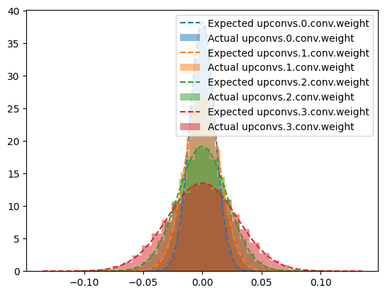
It initializes the weights from the upconv layers following the kaiming_normal_ algorithm in fan_in mode and nonlinearity set as ‘linear’, since no relu layer is used in the operation.

plot_param_dists(dec, 'upconvs\.\d\.conv\.weight', 1.)

for n, p in dec.named_parameters():
    if re.search('upconvs\.\d\.conv\.weight', n):
        fan_in = p.shape[1]*p.shape[2]*p.shape[3]
        mu, sigma = 0., np.sqrt(1./fan_in)
        p_data = p.view(-1).data
        assert abs(mu - p_data.mean()) < 1e-3
        assert abs(sigma - p_data.std()) < 1e-3

---

source

RIUNet

 RIUNet (in_channels=5, hidden_channels=(64, 128, 256, 512, 1024),
         n_classes=20)

RIU-Net complete architecture.

class RIUNet(Module):
    "RIU-Net complete architecture."
    def __init__(self, in_channels=5, hidden_channels=(64, 128, 256, 512, 1024), n_classes=20):
        super().__init__()
        self.n_classes = n_classes
        self.input_norm = BatchNorm2d(in_channels, affine=False, momentum=None)
        self.backbone = Sequential(OrderedDict([
            (f'enc', Encoder((in_channels, *hidden_channels))),
            (f'dec', Decoder(hidden_channels[::-1]))
        ]))
        self.head = Conv2d(hidden_channels[0], n_classes, 1)
        self.init_params()

    def init_params(self):
        for n, p in self.named_parameters():
            if re.search('head\.weight', n):
                normal_(p, std=1e-2)
            if re.search('head\.bias', n):
                zeros_(p)
    
    def forward(self, x):
        x = self.input_norm(x)
        features = self.backbone(x)
        prediction = self.head(features)
        
        return prediction

We slightly changed it to accept 5 input channels (i.e. x, y, z, depth and reflectance) instead of the 2 (depth and elevation) proposed in the original paper.

It implements the following architecture:

flowchart LR
  A(("
  Input
  (bs, 5, h, w)")) --> B["Encoder"]
  B --> C["Decoder"]
  C --> D["
  Conv(1x1)
  64 -> 20"]
  D --> E(("
  Output
  (bs, 20, h, w)"))

Here is an example on how to use it:

n_classes=20
model = RIUNet()
logits = model(inp)
assert logits.shape == (bs, n_classes, h, w)
print(logits.shape, f'== ({bs}, {n_classes}, {h}, {w})')

torch.Size([1, 20, 64, 512]) == (1, 20, 64, 512)

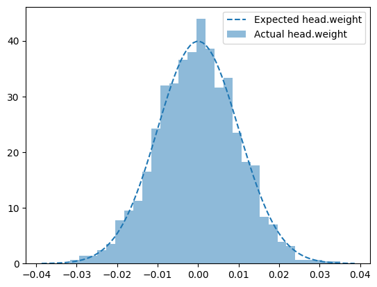
It initializes the weights from the classification head from a normal distribution with a standard deviation of 1e-2. The motivation is to reduce any random bias on the outputs of the untrained model.

plot_param_dists(model, 'head\.weight', 0.0064)

for n, p in model.named_parameters():
    if re.search('head\.weight', n):
        fan_in = p.shape[1]*p.shape[2]*p.shape[3]
        mu, sigma = 0., 1e-2
        p_data = p.view(-1).data
        assert abs(mu - p_data.mean()) < 1e-2
        assert abs(sigma - p_data.std()) < 1e-2

Loss function

The proposed equation for the loss function is the following.

\[ E = -\sum_{x \in \Omega}{w(x)\log(p_{l(x)}(x))\mathbf{1}_{\{m(x)>0\}}} \]

The factor \(w\) is motivated as a way “to give more importance to pixels that are close to a separation between two labels”. It was first defined in U-Net as follows.

\[ w(x) = w_c + w_{0}\exp\left ( -\frac{(d_{1}(x) + d_{2}(x))^{2}}{2\sigma^{2}} \right ) \]

From U-Net:

“where \(w_{c}\) […] is the weight map to balance the class frequencies, \(d_{1}\) […] denotes the distance to the border of the nearest cell and \(d_{2}\) […] the distance to the border of the second nearest cell.

While this particular equation for \(w\) can be seen as very specific for the original biomedical application in the Unet paper, its motivation is generally valid for any image semantic segmentation task such as ours. Hence, we can rewrite the equation for \(w\) as follows.

\[ w(x) = w_{c} + \lambda w_{b} \]

Similarly to the previous equation, \(w_{c}\) accounts for class imbalance, but the second term is rewritten as a general \(w_{b}\) factor that should account for the boundaries of the semantic maps.

For now, we only implemented the \(w_{c}\) factor. We leave the \(w_{b}\) factor and the necessary experimentation to evaluate its impact in the final model as TODO items.

Since the weighing and masking of the cross entropy loss is already implemented through the parameters weight and ignore_index in Pytorch’s CrossEntropyLoss module, we implement our own wrapper simply for convenience.

---

source

WeightedMaskedCELoss

 WeightedMaskedCELoss (weight, device)

Convenient wrapper for the CrossEntropyLoss module with a weight and ignore_index paremeters already set.

class WeightedMaskedCELoss(Module):
    "Convenient wrapper for the CrossEntropyLoss module with a `weight` and `ignore_index` paremeters already set."
    def __init__(self, weight, device):
        super().__init__()
        self.ignore_index = -1
        self.wmCE = CrossEntropyLoss(weight=torch.from_numpy(weight).to(device), ignore_index=self.ignore_index)

    def forward(self, pred, label, mask):
        label = label.clone()
        label[~mask] = self.ignore_index
        loss = self.wmCE(pred, label)
        return loss

Metrics

The proposed metric is the Intersection over Union (a.k.a. the Jaccard Index), which is implemented in the following module.

---

source

SegmentationIoU

 SegmentationIoU (num_classes, reduction='mean')

*Base class for all neural network modules.

Your models should also subclass this class.

Modules can also contain other Modules, allowing them to be nested in a tree structure. You can assign the submodules as regular attributes::

import torch.nn as nn
import torch.nn.functional as F

class Model(nn.Module):
    def __init__(self) -> None:
        super().__init__()
        self.conv1 = nn.Conv2d(1, 20, 5)
        self.conv2 = nn.Conv2d(20, 20, 5)

    def forward(self, x):
        x = F.relu(self.conv1(x))
        return F.relu(self.conv2(x))

Submodules assigned in this way will be registered, and will also have their parameters converted when you call :meth:to, etc.

.. note:: As per the example above, an __init__() call to the parent class must be made before assignment on the child.

:ivar training: Boolean represents whether this module is in training or evaluation mode. :vartype training: bool*

class SegmentationIoU(Module):
    def __init__(self, num_classes, reduction='mean'):
        assert reduction in ['mean', 'none']
        super().__init__()
        self.num_classes = num_classes
        self.reduction = reduction

    def forward(self, pred, label, mask):
        label = label.clone()
        pred[~mask] *= 0
        label[~mask] *= 0
        oh_pred = F.one_hot(pred, num_classes=self.num_classes)
        oh_label = F.one_hot(label, num_classes=self.num_classes)
        intersect = (oh_pred*oh_label).sum(dim=(1, 2))
        union = ((oh_pred + oh_label).clamp(max=1)).sum(dim=(1,2))
        intersect[union == 0] = 1
        union[union == 0] = 1
        iou = (intersect/union)
        if self.reduction == 'mean':
            iou = iou[:,1:].mean()
        return iou

SemanticKITTI Experiments

As mentioned in the summarizing quotes in the first section, the original experiments used “range-images with segmentation labels exported from the 3D object detection challenge of the KITTI dataset”. Improving on that, we implement our experiments using the SemanticKITTI: A Dataset for Semantic Scene Understanding of LiDAR Sequences, which was published around the same time as the RIU-Net paper and introduced a much bigger and better dataset for the task of pointcloud semantic segmentation.

Based on what was summarized from the Methodology and Experiments sections and our adaptations described in this notebook, here are the specifications of the Data, Model, Loss, Optimizer and Metric used in our experiments:

• Data:
  1. Applied spherical projection to 512 x 64 pixels
  2. 5 channels: x, y, z, reflectance, depth

from colorcloud.behley2019iccv import get_benchmarking_dls

dls = get_benchmarking_dls(
    data_path='/workspace/data',
    proj_style='spherical',
    proj_kargs={
        'fov_up_deg': 3., 
        'fov_down_deg': -25., 
        'W': 512, 'H': 64
    }
)

• Model:
  1. RIUNet module with its default hyperparameters

device = (
    "cuda"
    if torch.cuda.is_available()
    else "mps"
    if torch.backends.mps.is_available()
    else "cpu"
)
print(f"Using {device} device")

model = RIUNet().to(device)

• Loss:
  1. WeightedMaskedCELoss module

loss_fn = WeightedMaskedCELoss(dls[0].dataset.content_weights, device)

• Optimizer:
  1. AdamW with the OneCycleLR lr scheduler

lr = 1e-4
n_epochs = 30
total_steps = n_epochs*len(dls[0])

optimizer = AdamW(model.parameters(), lr)
lr_scheduler = OneCycleLR(optimizer, lr, total_steps)

• Metric:
  1. SegmentationIoU module

metric_fn = SegmentationIoU(dls[0].dataset.learning_map_np.max() + 1)

TODO: needs proper documentation with code examples for the experiments.